How To Predict Marginal Returns In Search

As a sequel to a previous post about “5 Steps To Leverage Those AdWords Bid Simulations For Maximum Return,” I wanted to shed some more light on the problem of predicting marginal returns in search marketing, as it is crucial to a successful paid search program — especially going into the Holiday season.

1. Estimate The Average Relationship Between Ad Spend & Revenue

At a high level, we first want to look at the current relationship between ad spend and revenue, and determine where we want to be in order to maximize ad revenue.

Note that your revenue or ROAS (return on ad spend) goal should not only reflect short-term online returns, i.e. what you can track currently, but also trailing revenue, returning revenue, cross-channel revenue, cross-device revenue, potentially in-store revenue, and anything else that make sense to your business.

So the relationship between ad spend and revenue (in a broad sense) can be based on historical weekly numbers, where you’d build a model such as “when I spent x in the past, I got y in revenue, and when I spent 2x, I got 1.5x in revenue,” and you should be able to determine a model which best fits how your program reacts with the ad spend using regression analysis.

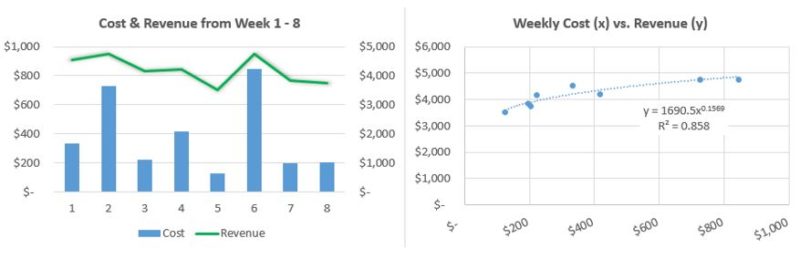
This type of approach works pretty well in a stable market, i.e., when there isn’t much volatility or any unusual market trends. Anyway, you can look at your weekly click, cost, and revenue data and translate those weekly trends in a general relationship between cost and revenue.

For instance, given the below weekly data points you saw from weeks 1 to 8, you can plot your cost (x) vs. revenue (y) and get to the conclusion that x dollars in ad spend bring y dollars in revenue. In this particular example I am using a power trend line and the model appears to be fitting fairly well.

In paid search, a similar but more granular approach is to use Google AdWords’ bid simulations, so that you get a sense of the relationship between max. CPC, clicks, cost, and revenue for each individual keyword in your account (except those low-volume or new keywords where those simulations are not available).

I won’t spend too much time explaining how to put together the data, as it is described in my previous post – but, long story short you should be able to put together the below table and yield curve quite easily by aggregating those AdWords’ bid simulations.

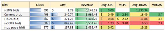
Note that the two yield curves we have now, one based on historical data, the other based on AdWords’ recent bid simulations, should look alike, however if they don’t, I’d personally tend to think your historical data was based due to seasonality.

2. Reiterate At The Keyword Level For Making Bid Decisions

While it is useful to know what is the general relationship between ad spend and revenue in order to allocate your budgets across channels, you still need to translate your overall objective (budget, ROAS, or marginal ROAS) into thousands or even millions of actionable keyword-level bids.

That is where it gets challenging, as you are going to need to further delve into the data to get to those optimal bids. More specifically, we are trying to answer the following question: what should my keywords’ individual bids be like so I spend $x on that particular day or week?

To answer that question, you can either analyze historical data at the keyword level, hoping most keywords got enough clicks, cost and revenue at different bid levels over time, or you can use AdWords’ simulations, or both together.

On a side note, I don’t personally need to use neither of those methods as the Adobe Media Optimizer platform provides simulations at the keyword level even for those low-volume or new keywords, however I feel it makes sense to illustrate the rationale of marginal returns through tools most people have easy access to, and that’d be AdWords of course.

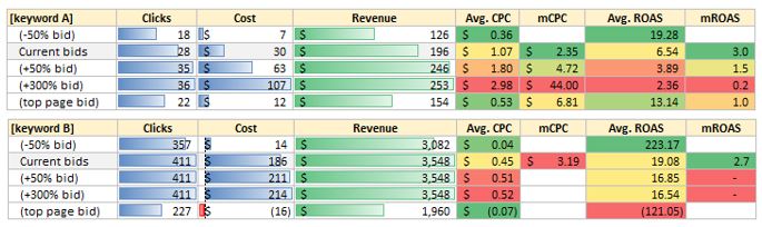
Getting back to our example, say we have two keywords: [keyword A] and [keyword B]. For [keyword A], those AdWords’ simulations indicate a marginal ROAS between 0.3 (if bidding +300%) up to 3.0 (if keeping the current bids). For [keyword B], we’re getting limited data as it is already in position 1.3, hence no incremental clicks when bidding up.

Now, if we want to determine what the bids should be across those two keywords in order to spend $x, we’re going to need to run a regression analysis for each individual keyword, similar to what we’ve done at a higher level previously.

Again, a power trend line worked well for me in this case, however, a power trend line is not always the best fit, so you should definitely try multiple regression types until you find the best fit.

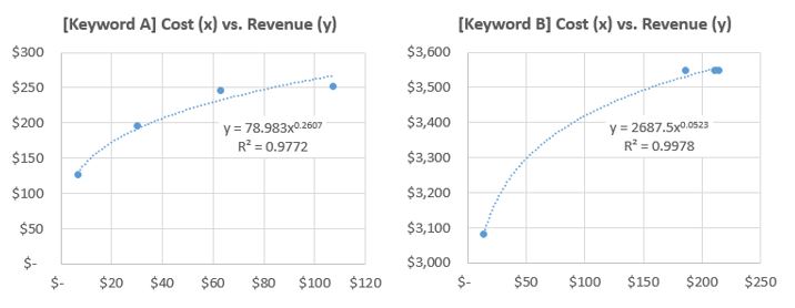
More specifically, if you want to spend $x the smartest way possible, you’ll want to align the mROAS (marginal return on ad spend) across keywords, so you’ll need to extrapolate the relationship between cost and revenue and look at the associated max CPCs and mROAS values. For instance:

So if you want to spend say $158, then the optimal Max CPCs for [keyword A] and [keyword B] would be $1.94 and $0.83 respectively, and a similar logic can be applied across millions of keywords – definitely not in Excel though!

3. Account For Seasonal Trends

Now let’s add a dimension to those data models: time. Essentially, we want to build the above models not only looking at recent data, but also at future days, weeks or months anticipating for changes in search volume, CPCs, and conversion rate. Indeed, our keywords A and B most likely behave quite differently over time.

So for each time period you need a prediction for, you can apply several factors such as in the below example: volume +30%, CPC +10%, conversion rate +20%, and you get to your estimated future yield curve based on your current yield curve.

More visually:

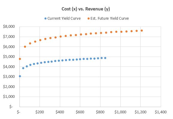
And you can repeat this process as many times as needed, then apply the previous logic to the keyword level in order to predict future max. CPCs based on your media plan in the next couple of weeks or months.

Conclusion

If you’ve read this post until here, then I’m sure you’ve realized how complex the process of analyzing historical data, building data models, and determining marginal ROAS-based bids can be.

And that was just for two keywords! Imagine how much more difficult things get when dealing with millions of keywords.

On top of that, complexity gets augmented when you begin to consider other bidding dimensions such as mobile bid adjustments, time of day bid adjustments, location bid adjustments, etc… Therefore, I truly believe in leveraging sophisticated technologies out there in order to scale this process and drive much greater results.