Polls And Testing: When Is Close No Cigar?

Now that the 2012 U.S. Presidential election is over, there’s a bit of buzz around why some folks thought the election would be close and others who, using some solid statistical techniques, predicted a definitive (and it turns out, accurate) outcome.

I want to try to explain the latter, especially for marketers. Why? Because political elections are in many ways like optimization testing: you’ve got two (or more) candidates and the “market” is choosing between them. So we can gain insight from understanding political polling that can assist us in our testing efforts and the metrics we use to judge them.

The Math-Lite Explanation

And, I’m going to attempt this without using much math. Why? Because many readers are marketers, and numbers can be… a challenge. You can always go dig up your local “small data” geek when you need to run such numbers yourself — so let’s focus on the concepts.

First off, to avoid the inevitable arguments of party affiliation, let us consider two fictional candidates, Mr. Smith and Ms. Jones. In the latest polls, Jones leads Smith 49 to 47 in a poll where the tiny print at the bottom of the results says there’s a margin of error of +/- 2 points.

First off, what do the above numbers mean? Based on a sampling of the voters, the simple answer is “Jones is slightly ahead (apparently).” You didn’t need a math whiz to derive that, although the “apparently” might seem odd.

Looking For “True” Numbers

As always, start with defining what metric we’re looking for. What we would really like are the “true” numbers — what the results will be on election day. That’s what we’re trying to predict or at least get a sense of. We are looking for which candidate is ahead at the time the poll is conducted as a means of guessing what the election outcome might be.

And again, for simplicity, we’ll leave out the discussion of polling bias, systemic bias, turn-out bias, etc., anything that might cause the people responding in the poll (the “sample” voters) to be anything other than completely representative of folks on election day (the “population” voters).

Now, a poll is just a snapshot in time; it’s not really a prediction for the (future) election day. But you can well imagine that as the polls get closer and closer to election day that they should, in principle, reflect closer and closer to what the end result turns out to be, at least as compared with polls taken many months earlier.

In the same way, if you’re running an A/B test on your site, you are hoping that the people responding to the test are approximately the same sort of customers as those who buy from you — usually true since the “control” variation is often the same as “how we currently do things” on your site. And, the equivalent of a “poll” is the snapshot of your A/B test when you’re part-way through the test.

What’s The Margin Of Error?

Back to Jones and Smith. What we know is this: a poll was conducted. Jones leads by two points. And there’s this odd “margin of error” number being thrown at us.

Now, since we’re really interested in is the outcome on election day, what we get from the margin of error is an estimate of where the true number for Jones and for Smith might be. A very common way to quote margin of error is at the 95% level. From the Jones-Smith poll, this means that Jones’ “true” number is somewhere in the range of 49% +/- 2% — that is, the true Jones number is somewhere between 47% and 51% (by the way, you will often see that range referred to as the “confidence interval”). Likewise, Smith is somewhere in the range 45% to 49% (47% +/- 2%).

And again, these are qualified as being “with 95% confidence.” All else being equal, if you did this poll a bunch of times, you’d certainly get slightly different numbers for Jones and Smith, but their true numbers would be outside the range above only about 1 time out of 20 (5%).

This is where most people stop. Hmm, wait a second, most people stop way before this! But, most folks who are interested stop right about at this point. But then you’d be missing all the interesting stuff to follow.

1) One important thing to keep in mind is that the margin of error, expressed as a percentage like +/- 2% above, is dependent on the number of people responding in the poll and how close the results are. The same results conducted over a larger number of people will mean a tighter margin of error.

A larger difference in the candidates (for example, say one candidate is way ahead) over the same number of people will mean a tighter margin of error (although in this case, it’s often more accurate to calculate margins of error for each candidate, but I digress).

In races that are relatively close, as in our Jones-Smith example, or in a country whose electorate is somewhat evenly split between two candidates, the margin begins to increase. In U.S. politics, the numbers for each side of the major party candidates are often in the 40s almost the entire election cycle, so that a particular poll’s margin of error is often just a function of the number of respondents in the poll. In this example, in the Jones-Smith poll there would have to have been a couple thousand people in the poll to get an m.o.e. of 2%

2) More importantly, just because Jones’ true number is somewhere in the range 49% +/- 2%, doesn’t mean it’s equally likely within that range. It’s much more likely for Jones to be at, say 50%, than for her to be at 51%. After all. the entire analysis is based on the assumption that we’re randomly sampling people when we do our poll. Also keep in mind that for Smith to be at 50% is way less likely than for Jones. This is an important part of what most people miss.

Yes, it’s absolutely possible for Smith to really be at 49%, the upper end of his confidence range, and for Jones to be at 47%, the lower end of her confidence range; but, that’s not nearly as likely than for Jones to be at 50 and Smith at 48.

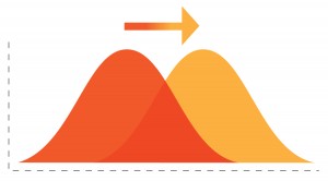
You might find it useful to think of it visually with Jones having a bell curve centered at 49%, and Smith having one centered at 47% (with the spread of each curve determined approximately by 2%/2). For Jones to win, her curve needs to be above Smith, which it is most of the time.

For Smith to win, he not only needs to get more of the vote than he is currently getting, but he must also get more of the vote than Jones, which is more of a challenge. So in this way, Jones really is further ahead than the spread between her and Smith, 49-47, superficially indicates.

The Monte Carlo Method

So, how would we go about estimating Jones’ chances to win? We know that voters in the poll are choosing her 49% to 47% for Smith. But 49% isn’t her probability of winning. That is determined by all the cases wherein she gets the most votes.

This is handled mathematically by something called a Monte Carlo method: we run the election based on these poll results and generate a random number, though as mentioned earlier, this is not equally random. You can roll snake eyes on a pair of dice, but the chances of rolling snake eyes is not the same as rolling, say, an eight. However, if you do this enough times you start to build up a probability curve for the expected results.

So, we repeat this simulation of running an election a hundred, or a thousand, or ten thousand times and look at all the results where Jones wins compared to where Smith wins. Professionals that number-crunch like this would typically use at least 100,000 runs. Given the numbers from our fictitious poll, what do you suppose the winning probability would be for Jones?

Pick a number in your head. Even odds of 50%? 60%? 75%? Write it down.

This is where the human part of the brain can lead one astray. If you saw numbers like that on your TV screen, one candidate ahead 49%-47%, you’d think “hmm, that’s somewhat of a close race; maybe the underdog can pull ahead.”

Turns out Jones is expected to win upwards of… wait for it… 96% of the time! Of course, the election is not run umpteen thousands of times; it’s only run once. So there’s definitely a chance for underdog Smith to win (about 4%, 1 in 25). And there’s always the probability that more of Smith people’s people will turn on on election day, etc., but according to the snapshot poll in our example, Jones looks pretty darn strong to take it.

It Only Seems Close

So, many times, things that are close are not really so. And, it’s extraordinarily easy to deceive oneself on these occasions. When you’re doing your A/B tests keep this in mind!

By the way, this use of the Monte Carlo technique is what Google Analytics Content Experiments (previously called Google Website Optimizer) used as a technique for “chance to beat” calculations.

P.S. I ran the simulations for our fictitious poll using a nifty program called R (which a numbers people love, but which might confuse the average marketer — use with adult supervision!)

Voting image used with permission from Shutterstock.